Speed up GJR-GARCH with Numba

June 1, 2019 | Michael Gong

Speed up GJR-GARCH with Numba

1. Introduction

GJR-GARCH is widely used for modeling the heteroskedasticity of assets’ return. GJR-GARCH introduces a asymmetric impact of the previous negative shocks at time $t$, which empirically turns out to outperforms the GARCH model.

The GJR-GARCH is defined as $$r_t = \mu + \epsilon_t$$ $$\epsilon_t=\sigma_t z_t$$

$$\sigma^2_t = \omega + \alpha\epsilon_t^2 + \gamma I_{t-1}\epsilon^2_{t-1} + \beta \sigma^2_{t-1}$$ where $I_{t-1} = 0$ if $r_{t-1}\geq \mu$, and $I_{t-1} = 1$ if $r_{t-1}<\mu$. The $r_t$ is the asset return, and $z_t$ is a standard Gaussian disturbance.

We usually estimate the parameters ${\mu, \omega,\alpha,\gamma,\beta }$ by minimize the negative log-likelihood function of the return process: $$LLF=-\frac{N}{2}\text{log}(2\pi)-\frac{1}{2}\sum_{t=1}^N\text{log}\sigma^2_t-\frac{1}{2}\sum_{t=1}^N\frac{\epsilon^2_t}{\sigma^2_t}$$

To compute the LLF, we need a forward pass of the GJR-GARCH process, which is slow in pure Python environment. If we have multiples assets and intend to back-test the performance with rolling window scheme, extreme long computation time might make the analysis infeasible. In this article, I show we can easily reduce the computation time with Numba’s Just-In-Time (JIT) compilation.

The code of this article requries pandas_datareader package (pip install pandas_datareader)

2. Prepare Data

import datetime as dt
import pandas_datareader.data as web
import matplotlib.pyplot as plt
%matplotlib inline

start = dt.datetime(2000, 1, 1)
end = dt.datetime(2019, 1, 1)
sp500 = web.DataReader('MSFT', 'yahoo', start=start, end=end)
returns = 100 * sp500['Adj Close'].pct_change().dropna()

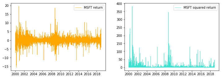
Plotting the return series and the squared return series, we can observe obvious volatility clustering

fig = plt.figure(figsize=(12,4))
ax = fig.add_subplot(1,2,1)
ax.plot(returns,label='MSFT return', linewidth=0.7, color="#ffa500")
plt.legend()
ax = fig.add_subplot(1,2,2)
ax.plot(returns**2,label='MSFT squared return', linewidth=0.7, color="#40e0d0")
plt.legend()

png

3. Pure Python GJR-GARCH implementation

import numpy as np
import pandas as pd

def garch_filter(omega, alpha, gamma, beta, eps):
    iT = len(eps)
    sigma_2 = np.zeros(iT)
    s = np.zeros(iT)
    
    # Setting the unconditional variance
    sigma_2[0] = omega/(1 - alpha - 0.5*gamma - beta)
    
    # Vectorize the asymmtric indicator
    s[eps<0] = 1
    
    # loop over the garch filter 
    for i in range(1, iT): 
        sigma_2[i] = omega + alpha * eps[i-1]**2 + gamma * s[i-1] * eps[i-1]**2 + beta*sigma_2[i-1]
    return sigma_2


def garch_loglike(mu, omega, alpha, gamma, beta, returns):
    iT = len(returns)
    eps = returns - mu
    sigma_2 = garch_filter(omega, alpha, gamma, beta, eps)
    loglike = ((iT/2 * np.log(2 * np.pi) + iT/2 * np.log(sigma_2[0]) + 1 /(2 * sigma_2[0]) * sum(eps ** 2)))

    return -loglike

4. Numba GJR-GARCH implementation

Once we set nopython=True, Numba will avoid python and compile the code using LLVM. So once the code is successfully compiled, we are no longer using the interpreted code, instead we are using compiled code.

from numba import jit

@jit(nopython=True)
def garch_filter(omega, alpha, gamma, beta, eps):
    iT = len(eps)
    sigma_2 = np.zeros(iT)
    s = np.zeros(iT)
    
    # Setting the unconditional variance
    sigma_2[0] = omega/(1 - alpha - 0.5*gamma - beta)
    
    # Vectorize the asymmtric indicator
    s[eps<0] = 1
    
    # loop over the garch filter 
    for i in range(1, iT): 
        sigma_2[i] = omega + alpha * eps[i-1]**2 + gamma * s[i-1] * eps[i-1]**2 + beta*sigma_2[i-1]
    return sigma_2


@jit(nopython=True)
def garch_loglikeJIT(mu, omega, alpha, gamma, beta, returns):
    iT = len(returns)
    eps = returns - mu
    sigma_2 = garch_filterJIT(omega, alpha, gamma, beta, eps)
    loglike = ((iT/2 * np.log(2 * np.pi) + iT/2 * np.log(sigma_2[0]) + 1 /(2 * sigma_2[0]) * np.sum(eps ** 2)))

    return -loglike

5. Performance comparison

vP0 = (1e-2, 1e-05, 0.1,0.15,0.8) # starting values
likelihood = garch_loglike(*vP0, returns.values)
likelihoodJIT = garch_loglikeJIT(*vP0, returns.values)
print(f"are the likelihoods the same? {likelihood==likelihoodJIT}")

are the likelihoods the same? True

Time the python garch filter

%timeit garch_loglike(*vP0, returns.values)

8.92 ms ± 71.1 µs per loop (mean ± std. dev. of 7 runs, 100 loops each)

TIme the numba garch filter

%timeit garch_loglikeJIT(*vP0, returns.values)

23.7 µs ± 127 ns per loop (mean ± std. dev. of 7 runs, 10000 loops each)

print(f"Speed up: {round(8920/23.7,2)}x")

Speed up: 376.37x

We obtain 376.37 speed-up by simply adding the Numba decorator!!!

6.Optimize the parameters

from scipy.optimize import approx_fprime, minimize

def optimizeHelper(vP, data):
#     vP = np.exp(vP)
    mu = vP[0]
    omega = vP[1]
    alpha = vP[2]
    gamma = vP[3]
    beta = vP[4]
    return -garch_loglikeJIT(mu, omega, alpha, gamma, beta, data)
    
nobs = len(returns.values)
vP0 = (1e-3, 1e-05, 0.15, 0.1,0.75)
func = lambda params: optimizeHelper(params, returns.values) / nobs
grad = lambda params: approx_fprime(params, func, 6.5e-7) / nobs
res = minimize(func, vP0, jac=grad, method = 'SLSQP', options={'ftol': 1e-10, 'maxiter': 200, 'disp':True})
print("Optimized parameters:",res.x)

Optimization terminated successfully.    (Exit mode 0)
            Current function value: 2.0767197604147474
            Iterations: 8
            Function evaluations: 18
            Gradient evaluations: 8
Optimized parameters: [     0.001      0.339      0.132      0.091      0.732]

mu, omega, alpha, gamma, beta = res.x
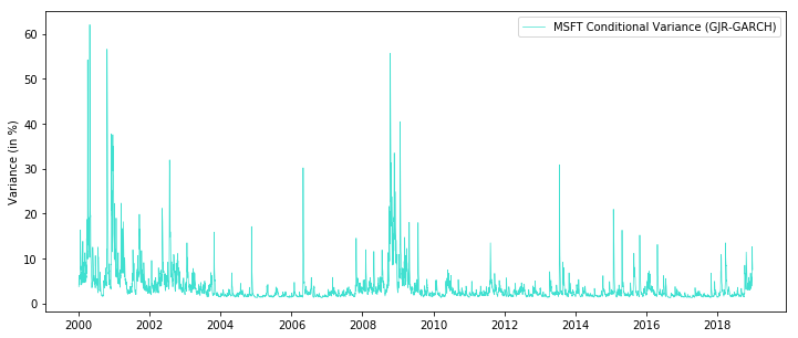
sigma2 = garch_filterJIT(omega, alpha, gamma, beta, returns.values- mu)

fig = plt.figure(figsize=(12,5))
ax = fig.add_subplot(111)
ax.plot(returns.index, sigma2, linewidth=0.7, color= "#40e0d0", label='MSFT Conditional Variance (GJR-GARCH)')
ax.set_ylabel('Variance (in %)')
plt.legend()

png